
The Current Expected Credit Losses standards (CECL) have once again been delayed for an undetermined period of time due to the Coronavirus Pandemic. Despite CECL implementation being pushed down the road again, forecasting credit losses is again front and center. This stems from the uncertainty created by the Pandemic and the nation’s corresponding response.
The debate and controversy surrounding CECL notwithstanding, the current situation we find ourselves in highlights an issue that plagues all modeling or forecasting. And that is unanticipated shocks. No matter what method is used to forecast credit losses, the primary takeaway from the current situation is the need for ancillary modeling and forecast methods to cope with a world that is increasingly governed by the unpredictable.
On Model Validity and Assumptions
In general, unexpected shocks undermine the validity of any model or forecast. The reason is simple, and we do not have to delve into theory or mathematics to understand it. The future is predicted in part by understanding the past combined with some assumptions about the future. Every prediction relies on assumptions. It often goes unrecognized, but these assumptions are the hinge upon which things turn and the typical place where models go wrong. Once the assumptions are set, the rest is just math.
If assumptions are 100% accurate, a model’s prediction will be accurate, assuming there are no calculation errors. Getting the math right is easy because it is finite and can be verified, whereas the assumptions usually cannot be. And, even if they could be verified, it does not eliminate the potential impact of the external shocks.
This crisis reinforces the need for institutions to have the ability to adjust and adapt to scenario- based forecast models. In a nutshell, lenders need a two-part tool kit. First, a benchmark forecast incorporating past trends and the current environment. This should be constantly expanding to encompass additional factors as well as be updated and maintained. Second, ancillary forecasting methods need to be available in order to respond to the unexpected.
At the risk of oversimplification, to illustrate our point, let’s consider where we are now and where we may be headed. We typically answer that question based on history. Although recent history has very little to offer in terms of data related to the Pandemic, one thing we may consider is economic data. Let’s start with the unemployment rate.
The unemployed rate as published by the Bureau of Labor Statistics was 4.4% in March. The more recent figure, April, is 14.7%. Immediately we notice that this is a stunning change. First, one would have to go back to 1940 to find a rate this high based on BLS data. Also, there does not appear to have ever been an increase of that magnitude in one month (except in the 1930’s).
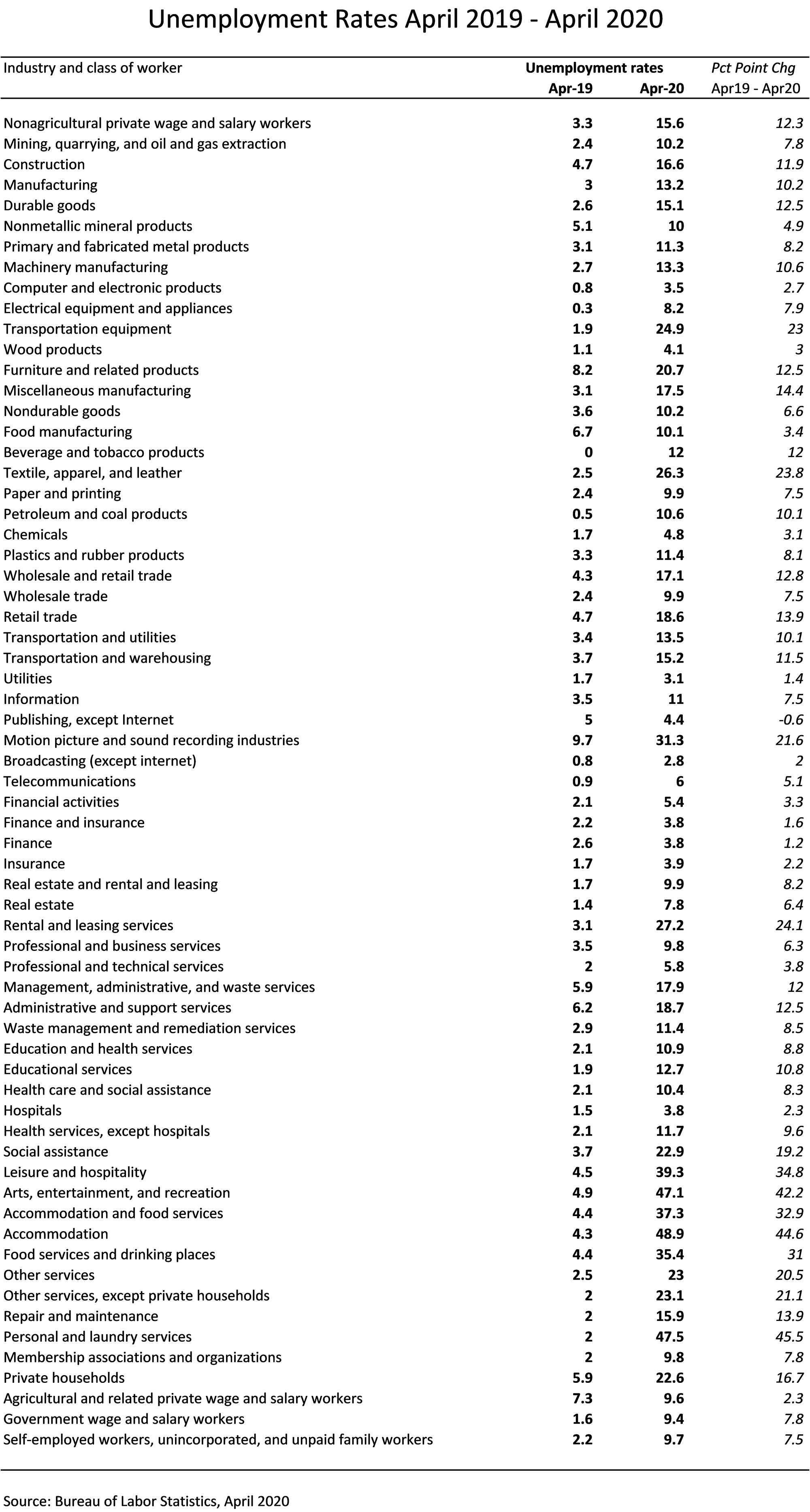
Delving a little deeper into the data, the table below shows unemployment rates from April and one year prior by industry. This shows which industries have been hit the hardest. As shown, some rates are close to 50% (arts and entertainment, accommodation, and personal and laundry services).
Along with the unemployment rate, another factor that is difficult to quantify but nevertheless should be considered is the stimulus bill passed by Congress. This consists largely of loan programs administered by banks and the Small Business Administration. The Payroll Protection Program (PPP) provided funds to businesses to pay employees, and the early guidance suggests that all or part of the loans are forgivable if used to cover payroll and certain operating costs. As part of the bill, consumers also received funds directly for assistance via stimulus checks.
While these programs provided needed relief to business and consumers, it, of course, comes at a price. These monies increase the federal debt and will have to be repaid at some point. The Fed also lowered the Fed Fund rate in response to the crisis so the government action will have both fiscal and monetary impacts.
Let’s now think of how we can apply these data. The unemployment rate seemingly gives us a stable measure and with much historical data with which to work. We also can look at loan losses and revenues over time relative to fluctuations in the unemployment rate.
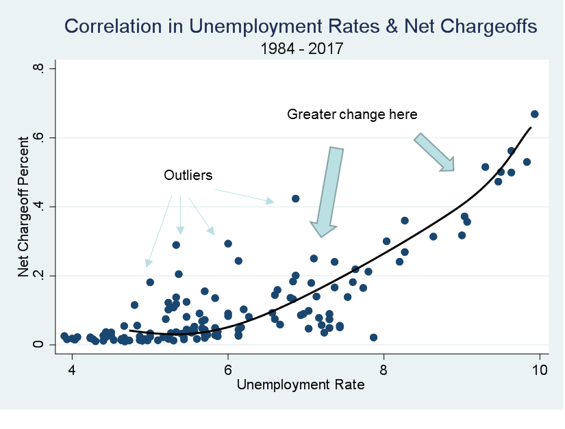
The graph below is an example. The net chargeoff rate is shown on the left side of the graph and the unemployment rate on the bottom of the graph. There are a number of things we can observe from these data.
First, as shown and as we would expect, losses tend to move with the unemployment rate. Aside from a few outliers that are noted on the graph, there appears to be a direct and positive relationship between the unemployment rate and net chargeoffs. As the unemployment rate increases, the rate of chargeoffs also increases.
We can also see that that the rate of change varies depending on the magnitude of the unemployment rate. Looking at the unemployment rate on the bottom of the graph, as the unemployment rate moves between 4% – 6%, there is a small increase in the rate of chargeoffs. However, from 6% – 8% there is a greater change, and then from 8% – 10% an even greater change. These sections are highlighted by the arrows shown on the graph.
Based on these data, we can visualize the change in expected losses based on changes in the unemployment rate.
Taking this a step further, we can quantify the expected change in the net chargeoff rates based on the increase in the unemployment rate. Using these data, which cover 1984 – 2017, the chargeoff rate would increase by 10 times based on the recent change in the unemployment rate. This would be a staggering number for lenders.
But would this be the appropriate adjustment for the ALLL estimate? The math would be correct. The data does indeed suggest that. But, right away there are at least three problems with respect to the assumptions.
Problem(s) When We Assume
Let’s examine these. The first one could be common to any forecast application, and that is out-of-sample prediction. In our data, the highest rate of unemployment is 9.9% when the current rate is 14.7%. The data goes back 30 years, so adding more data is probably not a good solution. But, trying to predict outside of the range of your data can be problematic in reliable forecasting.
The second issue is with respect to the government stimulus program. This undoubtedly will have some effect and has to be taken into account some way. Will it offset the impact of the unemployment rate? And if so, how much?
The third issue is what was discussed earlier, and that is lack of history applicable to the current situation. We have unemployment data with the rate of unemployment. However, the situation is anything but typical.
Usually, when the unemployment rate rises it occurs over a period of time and is related to the weakening of economic conditions. This is usually associated with adverse economic circumstances of some sort or some underlying issue that manifests in job losses. Here we had an abrupt increase in a matter of weeks that brought us to historically high levels. That in and of itself is very different. We have a number, but what this number means is uncertain.
Consider the most recent economic crisis, affectionately known as the “Great Recession.” The unemployment rate peaked at about 10%, but it took almost two years to get there. Too, the source of the problem was an asset bubble, and within months a tremendous amount of wealth was wiped out. This impacted business and consumers, leaving many in tough financial situations that persisted for years.
Again, our current situation is much different. Unlike previous downturns, this is not something that happened as much as it was something that was done. Guided by the federal government, the nation closed down a large portion of the economy. Not dissimilar to turning off a light switch. The GDP has fallen, and will likely fall more. But, GDP is largely a function of spending. Spending was curtailed by the voluntary shutdown as opposed to the typical situation in which spending erodes due to the lack of funds to spend.
The point here is that modern day complexities demand dynamic and adaptive approaches. The most important component of any forecasting model is the conceptual framework and the underlying assumptions. Even with a sound model and accurate assumptions, forecasts are usually taken at the means or averages. Averages or means are often referred to as “expected values” in statistics. In a global economy in which the trajectories are increasing determined by the unexpected, accuracy is a hefty expectation from a singular and static model. At the end of the day, a model is just a mathematical equation. BUT, the math is the easy part!